A reduced manuscript-style MBMM simulation

Purpose

This vignette provides a small, fully synthetic, end-to-end demonstration of the simulation structure used in the MBMM manuscript. It preserves the main scientific ingredients:

1. a continuous baseline antibody biomarker;
2. a biomarker-dependent latent productive-infection state;
3. productive viral-load trajectories generated from an eclipse-phase ODE;
4. nonestablishment trajectories that may contain transient or abortive detections;
5. irregular observation schedules, an assay limit of detection, and censoring;
6. MBMM fitting with a productive reference bank and an analytic nonestablishment model.

This is not a full reproduction of the manuscript simulation study. To keep package installation and checking practical, the vignette uses:

• fully synthetic antibody values;
• synthetic visit schedules;
• one small fixed productive reference bank;
• a reduced scenario grid;
• two illustrative replicates per scenario;
• asymptotic likelihood-ratio inference rather than permutation inference;
• MBMM and simple logistic summaries only.

The full manuscript study used empirically calibrated biomarker and visit distributions, a larger posterior bank, a substantially larger grid, comparator methods, permutation inference, and many Monte Carlo replicates. Therefore, the proportions shown below are illustrative run summaries, not estimates of power or type-I error.

Simulation ingredients

Synthetic baseline antibody

The public demonstration uses a bounded two-component Gaussian mixture on the natural-log scale. It produces a broad, right-skewed antibody distribution on the natural scale without including participant-level biomarker values.

set.seed(101)

antibody_demo <- mbmm_simulate_demo_antibody(
  n = 500,
  seed = 101
)

summary(
  antibody_demo[, c(
    "antibody",
    "log_antibody",
    "z_antibody"
  )]
)
#>     antibody       log_antibody     z_antibody     
#>  Min.   : 1.000   Min.   :0.000   Min.   :-2.2426  
#>  1st Qu.: 2.747   1st Qu.:1.011   1st Qu.:-0.7265  
#>  Median : 4.135   Median :1.420   Median :-0.1130  
#>  Mean   : 5.544   Mean   :1.495   Mean   : 0.0000  
#>  3rd Qu.: 7.591   3rd Qu.:2.027   3rd Qu.: 0.7981  
#>  Max.   :23.310   Max.   :3.149   Max.   : 2.4812

ggplot2::ggplot(
  antibody_demo,
  ggplot2::aes(x = antibody)
) +
  ggplot2::geom_histogram(
    bins = 30,
    fill = mbmm_palette[2],
    color = "white",
    linewidth = 0.2
  ) +
  ggplot2::labs(
    title = "Fully synthetic baseline antibody",
    x = "Antibody value (natural scale)",
    y = "Count"
  ) +
  theme_mbmm()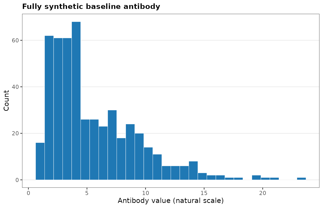

Productive-infection gate

For subject $i$, the latent productive-infection state is

$$Z_i \sim \operatorname{Bernoulli}(\pi_i), \qquad \operatorname{logit}(\pi_i) = \alpha + \beta x_i,$$

where $x_i$ is standardized baseline antibody. Negative $\beta$ represents a protective association. The simulation calibrates $\alpha$ so that the mean productive-infection probability across the realized synthetic biomarker distribution equals the requested target prevalence.

Transient and abortive patterns

A nonproductive subject may have one of four patterns:

• noise_like: no intended signal above the LOD;
• single_blip: one intended detectable visit;
• two_point: two intended near-LOD detections;
• fast_rise_drop: one higher isolated peak with neighboring visits remaining near background.

visit_days <- mbmm_demo_visit_schedules()[["complete"]]

abortive_examples <- do.call(
  rbind,
  lapply(
    c(
      "noise_like",
      "single_blip",
      "two_point",
      "fast_rise_drop"
    ),
    function(type) {
      x <- mbmm_simulate_abortive_pattern(
        times = visit_days,
        lod = 100,
        sigma_obs = 0.30,
        subtype = type,
        seed = match(
          type,
          c(
            "noise_like",
            "single_blip",
            "two_point",
            "fast_rise_drop"
          )
        ) + 200
      )
      x$pattern <- type
      x
    }
  )
)

abortive_examples$pattern <- factor(
  abortive_examples$pattern,
  levels = c(
    "noise_like",
    "single_blip",
    "two_point",
    "fast_rise_drop"
  )
)

abortive_plot_data <- abortive_examples
abortive_plot_data$y_plot <- pmax(abortive_plot_data$y, 1)

pattern_labels <- c(
  noise_like = "noise_like",
  single_blip = "single_blip",
  two_point = "two_point",
  fast_rise_drop = "fast_rise_drop"
)

lod_lines <- stats::aggregate(
  lod ~ pattern,
  data = abortive_plot_data,
  FUN = unique
)

ggplot2::ggplot(
  abortive_plot_data,
  ggplot2::aes(x = time, y = y_plot)
) +
  ggplot2::geom_hline(
    data = lod_lines,
    ggplot2::aes(yintercept = lod),
    linetype = mbmm_lod_linetype,
    color = mbmm_palette[7]
  ) +
  ggplot2::geom_line(color = mbmm_palette[2], linewidth = 0.5) +
  ggplot2::geom_point(color = mbmm_palette[2], size = 1.8) +
  ggplot2::scale_y_log10(limits = c(10, 5000)) +
  ggplot2::facet_wrap(
    ~pattern,
    labeller = ggplot2::as_labeller(pattern_labels)
  ) +
  ggplot2::labs(
    x = "Study day",
    y = "Observed viral load"
  ) +
  theme_mbmm()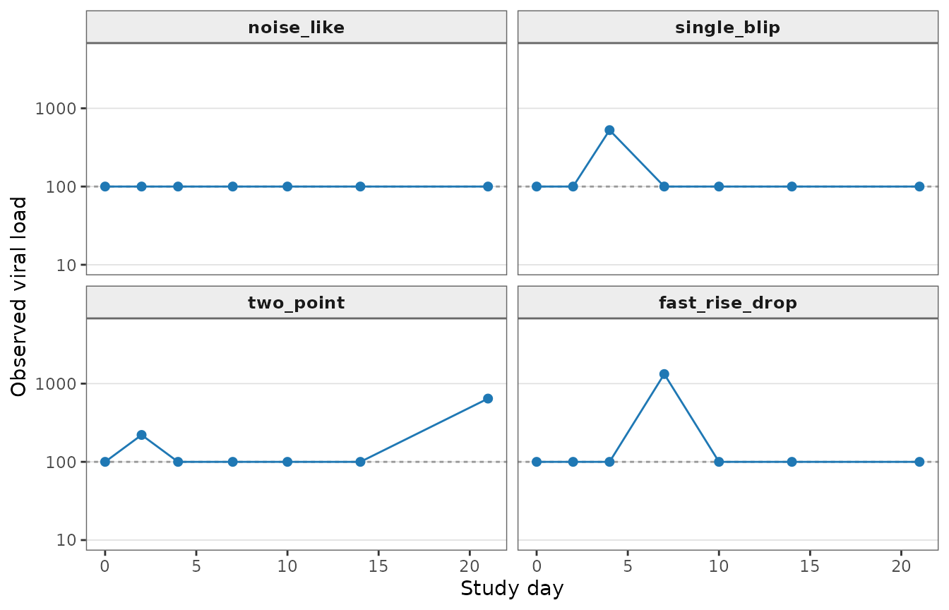

Build one small productive reference bank

The manuscript simulation reused a fixed productive reference bank. We follow the same structure here, but build a much smaller public bank from one synthetic reference cohort.

The ABC settings below are intentionally modest. They are suitable for a vignette demonstration, not for a substantive analysis.

reference_demo <- mbmm_simulate_manuscript_demo(
  n_subjects = 45,
  prevalence = 0.40,
  beta_true = 0,
  p_abortive = 0,
  n_bank_donors = 8,
  sigma_obs = 0.40,
  lod = 100,
  seed = 20260720
)

reference_ids <- reference_demo$subject_data$id[
  reference_demo$subject_data$bank_eligible
]

length(reference_ids)
#> [1] 8

abc_particles <- mbmm_abc_bank(
  obs_list = reference_demo$obs_list[reference_ids],
  simulate_fn = mbmm_example_eclipse_simulate,
  prior_sample_fn = mbmm_example_eclipse_prior,
  n_draws = 400,
  n_keep = 40,
  seed = 20260721,
  verbose = FALSE
)

pooled_productive <- mbmm_pool_bank(
  particles = abc_particles,
  seed = 20260722
)

prediction_times <- sort(
  unique(
    unlist(
      mbmm_demo_visit_schedules(),
      use.names = FALSE
    )
  )
)

productive_bank <- mbmm_predict_bank(
  bank = pooled_productive,
  simulate_fn = mbmm_example_eclipse_simulate,
  times = prediction_times
)

Reduced scenario grid

The demonstration uses:

• $N=50$;
• target productive prevalence $0.30$;
• $\beta \in \{0,-1.5\}$;
• abortive-event probability $p_A \in \{0,0.40\}$;
• two replicates per setting.

scenario_grid <- mbmm_demo_scenario_grid(
  replicates = 2,
  n_subjects = 50,
  prevalence = 0.30,
  beta_grid = c(0, -1.5),
  p_abortive_grid = c(0, 0.40),
  base_seed = 20260724
)

scenario_grid
#>   n_subjects prevalence beta_true p_abortive replicate                scenario
#> 1         50        0.3       0.0        0.0         1      beta=0; abortive=0
#> 2         50        0.3      -1.5        0.0         1   beta=-1.5; abortive=0
#> 3         50        0.3       0.0        0.4         1    beta=0; abortive=0.4
#> 4         50        0.3      -1.5        0.4         1 beta=-1.5; abortive=0.4
#> 5         50        0.3       0.0        0.0         2      beta=0; abortive=0
#> 6         50        0.3      -1.5        0.0         2   beta=-1.5; abortive=0
#> 7         50        0.3       0.0        0.4         2    beta=0; abortive=0.4
#> 8         50        0.3      -1.5        0.4         2 beta=-1.5; abortive=0.4
#>       seed
#> 1 20260724
#> 2 20260725
#> 3 20260726
#> 4 20260727
#> 5 20260728
#> 6 20260729
#> 7 20260730
#> 8 20260731

Run the reduced experiment

The helpers below extract coefficients and compute a simple AUC against the known latent state. Truth is used only for evaluating the simulation; it is not provided to the MBMM fitting functions.

extract_glm <- function(data, outcome) {
  y <- as.integer(data[[outcome]])

  if (length(unique(y)) < 2L) {
    return(
      c(
        beta = NA_real_,
        p_value = NA_real_
      )
    )
  }

  fit <- suppressWarnings(
    stats::glm(
      y ~ baseline_antibody,
      data = data,
      family = stats::binomial()
    )
  )

  tab <- summary(fit)$coefficients

  c(
    beta = unname(tab["baseline_antibody", "Estimate"]),
    p_value = unname(tab["baseline_antibody", "Pr(>|z|)"])
  )
}


auc_binary <- function(score, truth) {
  truth <- as.integer(truth)
  n1 <- sum(truth == 1L)
  n0 <- sum(truth == 0L)

  if (
    n1 == 0L ||
      n0 == 0L ||
      length(score) != length(truth) ||
      any(!is.finite(score))
  ) {
    return(NA_real_)
  }

  ranks <- rank(score)

  (
    sum(ranks[truth == 1L]) -
      n1 * (n1 + 1) / 2
  ) / (n1 * n0)
}


extract_gate_beta <- function(gate, term = "baseline_antibody") {
  row <- gate$coef[
    gate$coef$term == term,
    ,
    drop = FALSE
  ]

  if (nrow(row) != 1L) {
    return(NA_real_)
  }

  as.numeric(row$estimate)
}

simulation_runs <- mbmm_run_simulation_grid(
  grid = scenario_grid,
  productive_bank = productive_bank,
  n_cores = 1
)

simulation_results <- do.call(
  rbind,
  lapply(
    simulation_runs,
    function(x) {
      fit <- x$fit
      demo <- x$demo
      setting <- x$setting

      oracle <- extract_glm(
        demo$subject_data,
        outcome = "productive_true"
      )

      logistic_any <- extract_glm(
        demo$subject_data,
        outcome = "any_detect"
      )

      logistic_two <- extract_glm(
        demo$subject_data,
        outcome = "two_detect"
      )

      posterior <- merge(
        fit$gate$posterior,
        demo$subject_data[
          ,
          c(
            "id",
            "productive_true",
            "true_class"
          )
        ],
        by = "id",
        all.x = TRUE,
        sort = FALSE
      )

      beta_mbmm <- extract_gate_beta(
        fit$gate
      )

      data.frame(
        scenario = setting$scenario,
        replicate = setting$replicate,
        seed = setting$seed,
        n_subjects = setting$n_subjects,
        prevalence = setting$prevalence,
        beta_true = setting$beta_true,
        p_abortive = setting$p_abortive,
        n_productive = sum(
          demo$subject_data$productive_true
        ),
        realized_productive_fraction = mean(
          demo$subject_data$productive_true
        ),
        observed_any_detect_fraction = mean(
          demo$subject_data$any_detect
        ),
        observed_two_detect_fraction = mean(
          demo$subject_data$two_detect
        ),
        beta_oracle = unname(
          oracle["beta"]
        ),
        p_oracle = unname(
          oracle["p_value"]
        ),
        beta_logistic_any = unname(
          logistic_any["beta"]
        ),
        p_logistic_any = unname(
          logistic_any["p_value"]
        ),
        beta_logistic_two = unname(
          logistic_two["beta"]
        ),
        p_logistic_two = unname(
          logistic_two["p_value"]
        ),
        beta_mbmm = beta_mbmm,
        lrt_mbmm = as.numeric(
          fit$gate$LRT
        ),
        p_mbmm = as.numeric(
          fit$gate$p_value
        ),
        sig_mbmm =
          is.finite(fit$gate$p_value) &&
          fit$gate$p_value < 0.05 &&
          is.finite(beta_mbmm) &&
          beta_mbmm < 0,
        auc_mbmm = auc_binary(
          posterior$posterior_productive,
          posterior$productive_true
        ),
        optimizer_ok =
          identical(
            fit$gate$convergence_full,
            0L
          ) &&
          identical(
            fit$gate$convergence_null,
            0L
          ),
        stringsAsFactors = FALSE
      )
    }
  )
)

rownames(simulation_results) <- NULL

example_fits <- lapply(
  simulation_runs,
  function(x) {
    posterior <- merge(
      x$fit$gate$posterior,
      x$demo$subject_data[
        ,
        c(
          "id",
          "productive_true",
          "true_class"
        )
      ],
      by = "id",
      all.x = TRUE,
      sort = FALSE
    )

    list(
      setting = x$setting,
      demo = x$demo,
      fit = x$fit,
      posterior = posterior
    )
  }
)

simulation_results
#>                  scenario replicate     seed n_subjects prevalence beta_true
#> 1      beta=0; abortive=0         1 20260724         50        0.3       0.0
#> 2   beta=-1.5; abortive=0         1 20260725         50        0.3      -1.5
#> 3    beta=0; abortive=0.4         1 20260726         50        0.3       0.0
#> 4 beta=-1.5; abortive=0.4         1 20260727         50        0.3      -1.5
#> 5      beta=0; abortive=0         2 20260728         50        0.3       0.0
#> 6   beta=-1.5; abortive=0         2 20260729         50        0.3      -1.5
#> 7    beta=0; abortive=0.4         2 20260730         50        0.3       0.0
#> 8 beta=-1.5; abortive=0.4         2 20260731         50        0.3      -1.5
#>   p_abortive n_productive realized_productive_fraction
#> 1        0.0           18                         0.36
#> 2        0.0           13                         0.26
#> 3        0.4           13                         0.26
#> 4        0.4           14                         0.28
#> 5        0.0            9                         0.18
#> 6        0.0           14                         0.28
#> 7        0.4           14                         0.28
#> 8        0.4           16                         0.32
#>   observed_any_detect_fraction observed_two_detect_fraction beta_oracle
#> 1                         0.48                         0.34  -0.4564197
#> 2                         0.36                         0.26  -1.1036590
#> 3                         0.48                         0.36  -0.1163806
#> 4                         0.48                         0.36  -2.6632927
#> 5                         0.28                         0.18  -0.4678926
#> 6                         0.34                         0.24  -1.2424223
#> 7                         0.62                         0.34  -0.2074081
#> 8                         0.52                         0.36  -1.2125405
#>       p_oracle beta_logistic_any p_logistic_any beta_logistic_two
#> 1 0.1446159346        -0.2347796    0.418927651       -0.49827953
#> 2 0.0105232252        -0.7517430    0.029010457       -1.10365899
#> 3 0.7239473393        -0.2304127    0.427670598       -0.05097333
#> 4 0.0009930458        -1.0381037    0.007307308       -1.53667148
#> 5 0.2325487711        -0.6016627    0.085267022       -0.46789255
#> 6 0.0038433740        -1.3089872    0.001652013       -1.30928097
#> 7 0.5219066114         0.6944448    0.041182984        0.45806542
#> 8 0.0038841025        -0.7049039    0.033355559       -0.96363239
#>   p_logistic_two  beta_mbmm   lrt_mbmm       p_mbmm sig_mbmm  auc_mbmm
#> 1    0.118996610 -0.4621338  2.2876241 1.304094e-01    FALSE 1.0000000
#> 2    0.010523225 -1.1036387  8.5537205 3.448168e-03     TRUE 1.0000000
#> 3    0.864387515 -0.1163644  0.1258456 7.227789e-01    FALSE 1.0000000
#> 4    0.002136126 -1.8668765 17.5136758 2.852485e-05     TRUE 0.9960317
#> 5    0.232548771 -0.2115440  0.2850289 5.934239e-01    FALSE 1.0000000
#> 6    0.005034332 -1.2526364 10.8538290 9.859169e-04     TRUE 0.9543651
#> 7    0.149614004 -0.2074060  0.4166568 5.186100e-01    FALSE 1.0000000
#> 8    0.009521418 -1.1114412  9.8747350 1.675637e-03     TRUE 1.0000000
#>   optimizer_ok
#> 1         TRUE
#> 2         TRUE
#> 3         TRUE
#> 4         TRUE
#> 5         TRUE
#> 6         TRUE
#> 7         TRUE
#> 8         TRUE

parallel_runs <- mbmm_run_simulation_grid(
  grid = scenario_grid,
  productive_bank = productive_bank,
  n_cores = 2
)

Scenario summaries

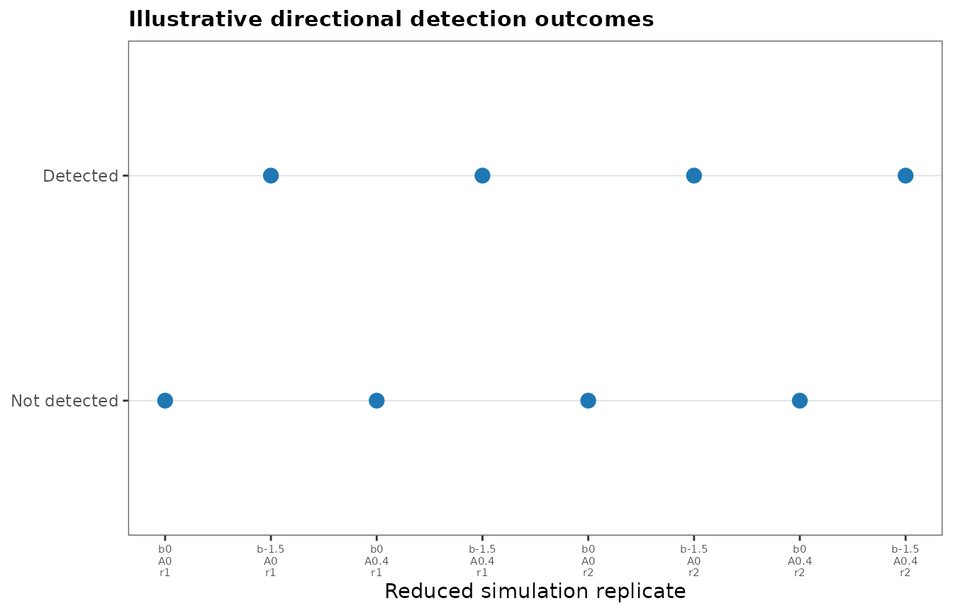
With only two replicates per setting, the detection proportion below should not be interpreted as statistical power.

split_results <- split(
  simulation_results,
  interaction(
    simulation_results$beta_true,
    simulation_results$p_abortive,
    drop = TRUE
  )
)

scenario_summary <- do.call(
  rbind,
  lapply(
    split_results,
    function(x) {
      data.frame(
        beta_true = unique(x$beta_true),
        p_abortive = unique(x$p_abortive),
        replicates = nrow(x),
        mean_beta_mbmm = mean(
          x$beta_mbmm,
          na.rm = TRUE
        ),
        mean_beta_bias = mean(
          x$beta_mbmm - x$beta_true,
          na.rm = TRUE
        ),
        illustrative_detection_fraction = mean(
          x$sig_mbmm,
          na.rm = TRUE
        ),
        mean_auc_mbmm = mean(
          x$auc_mbmm,
          na.rm = TRUE
        ),
        optimizer_success_fraction = mean(
          x$optimizer_ok,
          na.rm = TRUE
        ),
        stringsAsFactors = FALSE
      )
    }
  )
)

rownames(scenario_summary) <- NULL

scenario_summary
#>   beta_true p_abortive replicates mean_beta_mbmm mean_beta_bias
#> 1      -1.5        0.0          2     -1.1781375     0.32186246
#> 2       0.0        0.0          2     -0.3368389    -0.33683888
#> 3      -1.5        0.4          2     -1.4891589     0.01084112
#> 4       0.0        0.4          2     -0.1618852    -0.16188516
#>   illustrative_detection_fraction mean_auc_mbmm optimizer_success_fraction
#> 1                               1     0.9771825                          1
#> 2                               0     1.0000000                          1
#> 3                               1     0.9980159                          1
#> 4                               0     1.0000000                          1

Manuscript-style figures

Example productive and transient/abortive trajectories

The figure below displays one simulated dataset from the protective, high-abortive setting. Curves are grouped by the known generating phenotype for illustration.

example_index <- which(
  scenario_grid$beta_true == -1.5 &
    scenario_grid$p_abortive == 0.40 &
    scenario_grid$replicate == 1
)[1]

trajectory_demo <- example_fits[[example_index]]$demo

selected_ids <- c(
  head(
    trajectory_demo$subject_data$id[
      trajectory_demo$subject_data$true_class == "productive"
    ],
    4
  ),
  head(
    trajectory_demo$subject_data$id[
      trajectory_demo$subject_data$abortive_subtype == "single_blip"
    ],
    2
  ),
  head(
    trajectory_demo$subject_data$id[
      trajectory_demo$subject_data$abortive_subtype == "two_point"
    ],
    2
  ),
  head(
    trajectory_demo$subject_data$id[
      trajectory_demo$subject_data$abortive_subtype == "fast_rise_drop"
    ],
    2
  )
)

trajectory_plot_data <- merge(
  trajectory_demo$observations[
    trajectory_demo$observations$id %in% selected_ids,
    ,
    drop = FALSE
  ],
  trajectory_demo$subject_data[
    ,
    c(
      "id",
      "true_class",
      "abortive_subtype"
    )
  ],
  by = "id",
  all.x = TRUE
)

trajectory_plot_data$display_class <- ifelse(
  trajectory_plot_data$true_class == "productive",
  "productive",
  trajectory_plot_data$abortive_subtype
)

trajectory_plot_data$y_plot <- pmax(trajectory_plot_data$y, 1)
trajectory_plot_data$id <- factor(trajectory_plot_data$id)

class_colors <- stats::setNames(
  mbmm_palette[c(2, 5, 4, 3)],
  c("productive", "single_blip", "two_point", "fast_rise_drop")
)

lod_lines_traj <- stats::aggregate(
  lod ~ display_class,
  data = trajectory_plot_data,
  FUN = function(x) unique(x)[1]
)

ggplot2::ggplot(
  trajectory_plot_data,
  ggplot2::aes(x = time, y = y_plot, group = id)
) +
  ggplot2::geom_hline(
    data = lod_lines_traj,
    ggplot2::aes(yintercept = lod),
    linetype = mbmm_lod_linetype,
    color = mbmm_palette[7]
  ) +
  ggplot2::geom_line(
    ggplot2::aes(color = display_class),
    linewidth = 0.5,
    alpha = 0.9
  ) +
  ggplot2::geom_point(
    ggplot2::aes(color = display_class),
    size = 1.8
  ) +
  ggplot2::scale_y_log10() +
  ggplot2::scale_color_manual(values = class_colors, guide = "none") +
  ggplot2::facet_wrap(~display_class, ncol = 2) +
  ggplot2::labs(
    x = "Study day",
    y = "Observed viral load"
  ) +
  theme_mbmm()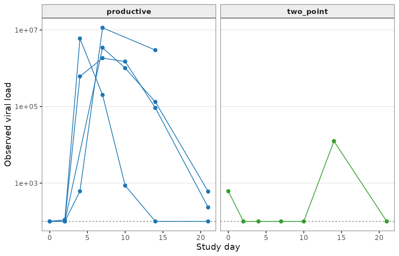

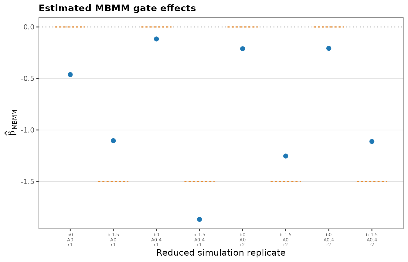
Estimated gate effects

Each point represents one reduced simulation replicate. Horizontal segments show the true generating effect for each setting.

effect_plot_data <- simulation_results
effect_plot_data$replicate_index <- seq_len(nrow(effect_plot_data))
effect_plot_data$x_label <- paste0(
  "b", effect_plot_data$beta_true,
  "\nA", effect_plot_data$p_abortive,
  "\nr", effect_plot_data$replicate
)

ggplot2::ggplot(
  effect_plot_data,
  ggplot2::aes(x = replicate_index, y = beta_mbmm)
) +
  ggplot2::geom_hline(
    yintercept = 0,
    linetype = "13",
    color = mbmm_palette[7]
  ) +
  ggplot2::geom_segment(
    ggplot2::aes(
      x = replicate_index - 0.35,
      xend = replicate_index + 0.35,
      y = beta_true,
      yend = beta_true
    ),
    linetype = mbmm_lod_linetype,
    color = mbmm_palette[3],
    linewidth = 0.6
  ) +
  ggplot2::geom_point(color = mbmm_palette[2], size = 2.2) +
  ggplot2::scale_x_continuous(
    breaks = effect_plot_data$replicate_index,
    labels = effect_plot_data$x_label
  ) +
  ggplot2::labs(
    title = "Estimated MBMM gate effects",
    x = "Reduced simulation replicate",
    y = expression(hat(beta)[MBMM])
  ) +
  theme_mbmm() +
  ggplot2::theme(
    axis.text.x = ggplot2::element_text(size = ggplot2::rel(0.65))
  )

Illustrative detection outcomes

Filled points indicate a directional MBMM result with $p<0.05$ and a negative estimated biomarker effect.

detection_plot_data <- simulation_results
detection_plot_data$replicate_index <- seq_len(nrow(detection_plot_data))
detection_plot_data$x_label <- paste0(
  "b", detection_plot_data$beta_true,
  "\nA", detection_plot_data$p_abortive,
  "\nr", detection_plot_data$replicate
)
detection_plot_data$outcome <- factor(
  ifelse(detection_plot_data$sig_mbmm, "Detected", "Not detected"),
  levels = c("Not detected", "Detected")
)

ggplot2::ggplot(
  detection_plot_data,
  ggplot2::aes(x = replicate_index, y = outcome, shape = outcome)
) +
  ggplot2::geom_point(
    color = mbmm_palette[2],
    fill = mbmm_palette[2],
    size = 2.6,
    stroke = 1
  ) +
  ggplot2::scale_shape_manual(
    values = c("Not detected" = 21, "Detected" = 19),
    guide = "none"
  ) +
  ggplot2::scale_x_continuous(
    breaks = detection_plot_data$replicate_index,
    labels = detection_plot_data$x_label
  ) +
  ggplot2::labs(
    title = "Illustrative directional detection outcomes",
    x = "Reduced simulation replicate",
    y = NULL
  ) +
  theme_mbmm() +
  ggplot2::theme(
    axis.text.x = ggplot2::element_text(size = ggplot2::rel(0.65))
  )

Posterior phenotype discrimination

For one illustrative protective, high-abortive dataset, the posterior productive probability is shown against the true latent class.

posterior_example <- example_fits[[example_index]]$posterior
posterior_example$true_class_label <- factor(
  posterior_example$productive_true,
  levels = c(0, 1),
  labels = c("Nonestablishment", "Productive")
)

ggplot2::ggplot(
  posterior_example,
  ggplot2::aes(x = true_class_label, y = posterior_productive)
) +
  ggplot2::geom_boxplot(
    ggplot2::aes(fill = true_class_label),
    outlier.shape = NA,
    alpha = 0.35,
    width = 0.55
  ) +
  ggplot2::geom_jitter(
    ggplot2::aes(color = true_class_label),
    width = 0.12,
    height = 0,
    size = 1.8,
    alpha = 0.85
  ) +
  ggplot2::scale_fill_manual(
    values = c(
      "Nonestablishment" = mbmm_palette[6],
      "Productive" = mbmm_palette[2]
    ),
    guide = "none"
  ) +
  ggplot2::scale_color_manual(
    values = c(
      "Nonestablishment" = mbmm_palette[6],
      "Productive" = mbmm_palette[2]
    ),
    guide = "none"
  ) +
  ggplot2::labs(
    title = "Illustrative phenotype discrimination",
    x = "True latent class",
    y = "Posterior productive probability"
  ) +
  theme_mbmm()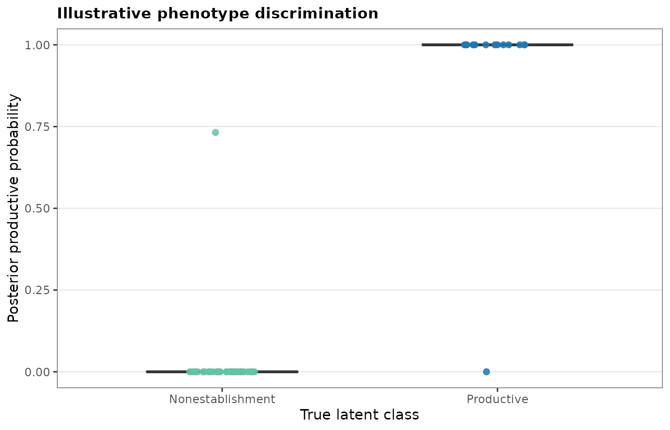

Scaling toward the manuscript experiment

The following chunk is not evaluated. It illustrates the kinds of settings that must be increased for a larger reproduction. Replace the placeholder values with the exact manuscript and supplementary-code settings.

full_grid <- expand.grid(
  n_subjects = c(25, 40, 50, 75, 100, 150, 200),
  prevalence = c(0.20, 0.30),
  beta_true = c(0, -0.5, -1.0, -1.5),
  p_abortive = c(0, 0.20, 0.40),
  replicate = seq_len(100)
)

# Increase these settings for a substantive analysis.
abc_n_draws <- 10000
abc_accept_fraction <- 0.025
n_permutations <- 199

# The full manuscript workflow additionally included comparator methods,
# checkpointing, parallel execution, and manuscript-specific summaries.

A full reproduction should also restore:

• the empirically calibrated biomarker distribution, where permitted;
• the empirical visit-pattern distribution, where permitted;
• the full productive posterior bank;
• all sample-size, prevalence, effect-size, and abortive-event settings;
• the planned number of Monte Carlo replicates;
• permutation inference;
• the manuscript comparator methods;
• the exact manuscript figure-generation scripts.

Interpretation

This vignette is designed to verify the public package workflow and make the simulation architecture transparent. It demonstrates that MBMM can be run end-to-end when PCR-detectable transient or abortive events do not necessarily represent productive infection.

The numerical results from this small vignette should not be quoted as formal power, type-I error, or performance estimates.